Visualising Convolution in CT through Mathematica

The following code can be used to convolve signals x(t) and h(t) and plot them in an interactive way.

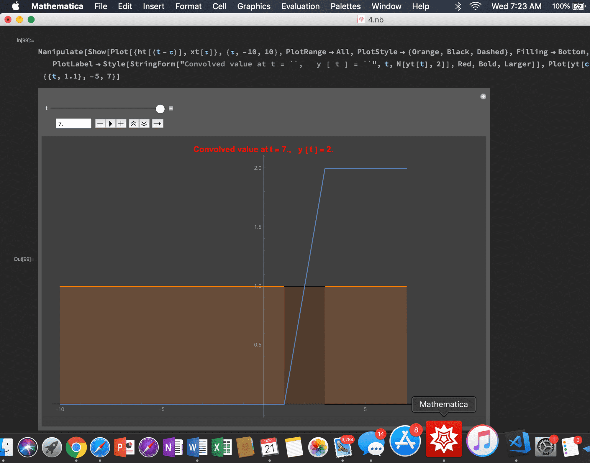
The blue curve represents the convolved signal y(t) at t, while other two are x(t) and h(t). In this example h(t) is the UnitStep Function. Therefore overall the system behaves as an Accumulator.

My code is given below. You can do experiments by changing the impulse response h(t) and visualising y(t) which is the convolved signal. The animation shows the steps in convolution,

Flip ‣ Shift (about y axis) (orange curve) ‣ Multiply ‣ Sum

Mathematica code : (click to open in full)

you will need to download and run the code [ *.nb file ] because there may be issues running the code live on the browser.

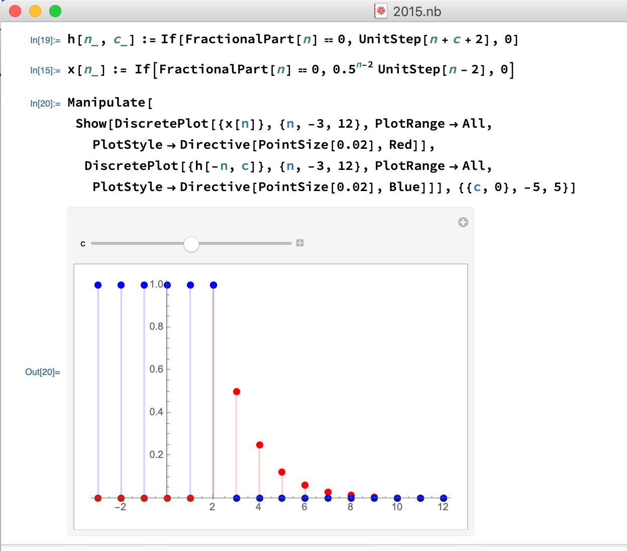
This code can be further modified to compute convolution in Discrete Time. If you're interested, please let me know in the comments below, and I'll write a separate article on it.

Next Steps. -> In discrete time